
Intro
I wanted to build a CNC microscope using off the shelf parts in order to attempt image fairly large objects such leaves, CD-ROMs etc. to reveal detail that can’t be seen with the naked eye.
This required a metallurgical style microscope, which shines light through a microscope objective, onto a sample.
Initial attempt
I initially attempted to fix the microscope in place using a rather large amount of plasticine. This did hold it in place for a little while, until it began to creep and fall through!
To fit the microscope through the tool holder I had to first unscrew the mirror section of the microscope and re-install after.
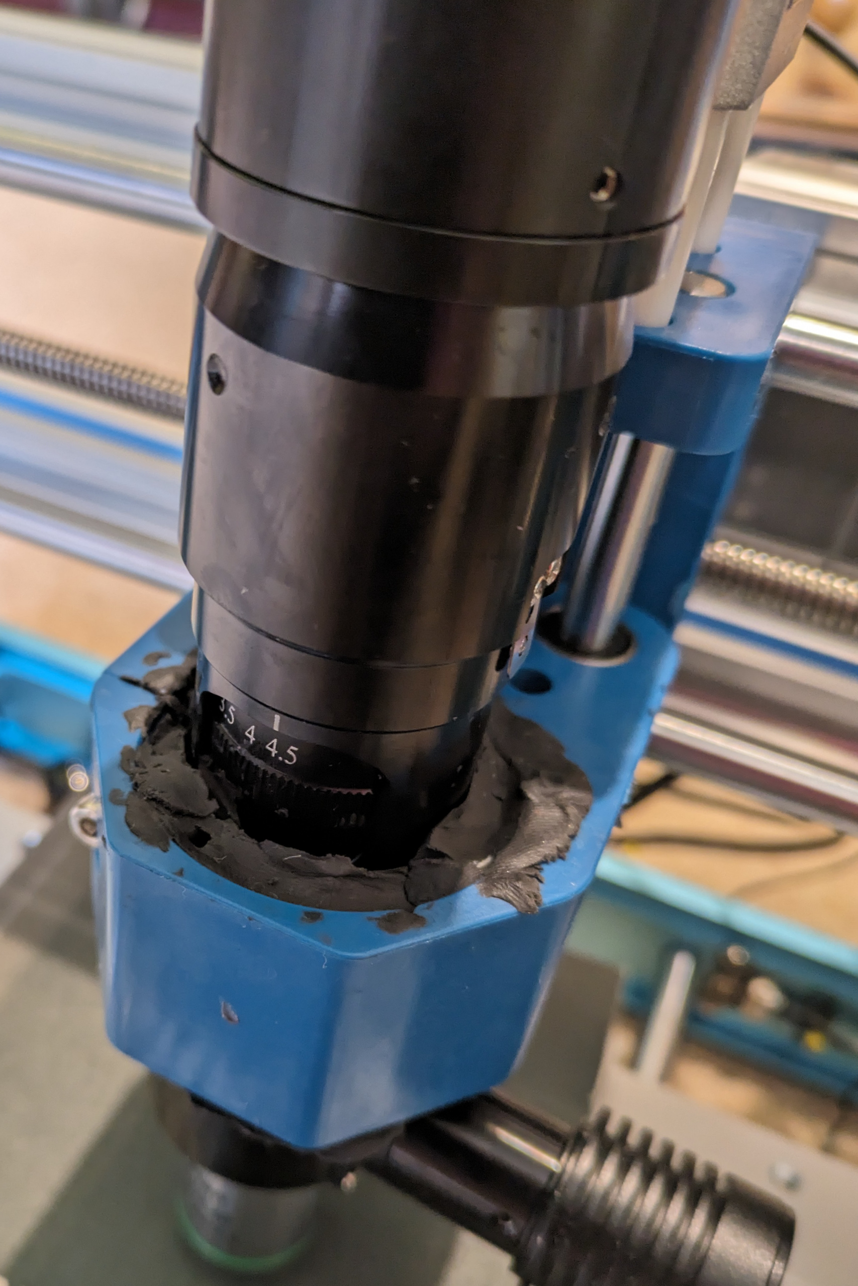
I switched from plasticine to neoprene tape, which held the microscope in place much more effectively!
To install the microscope I wrapped it with the neoprene tape and unscrewed the CNC’s tool holder and gently prised it wide open to install the scope and re-install the screw.
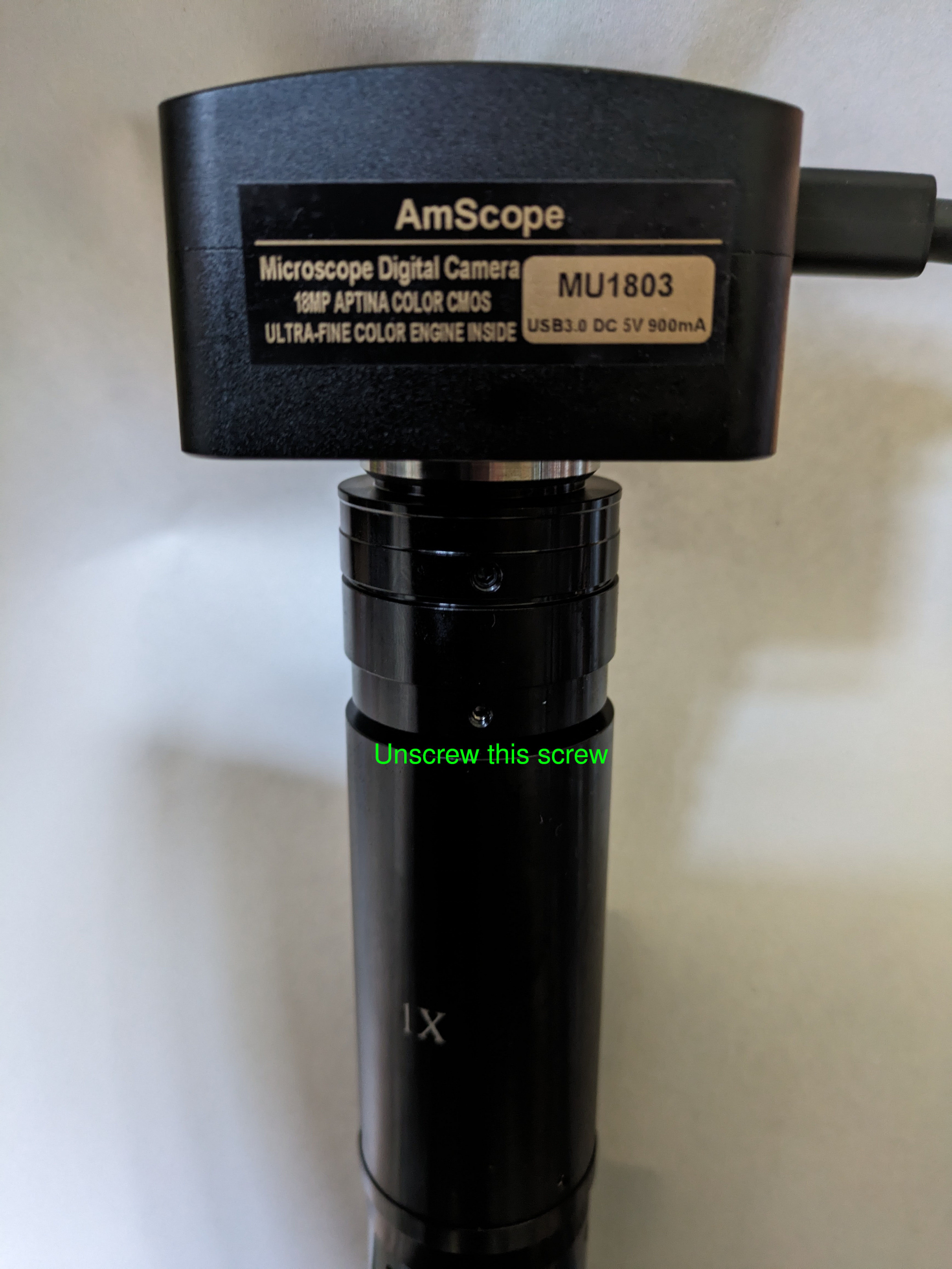
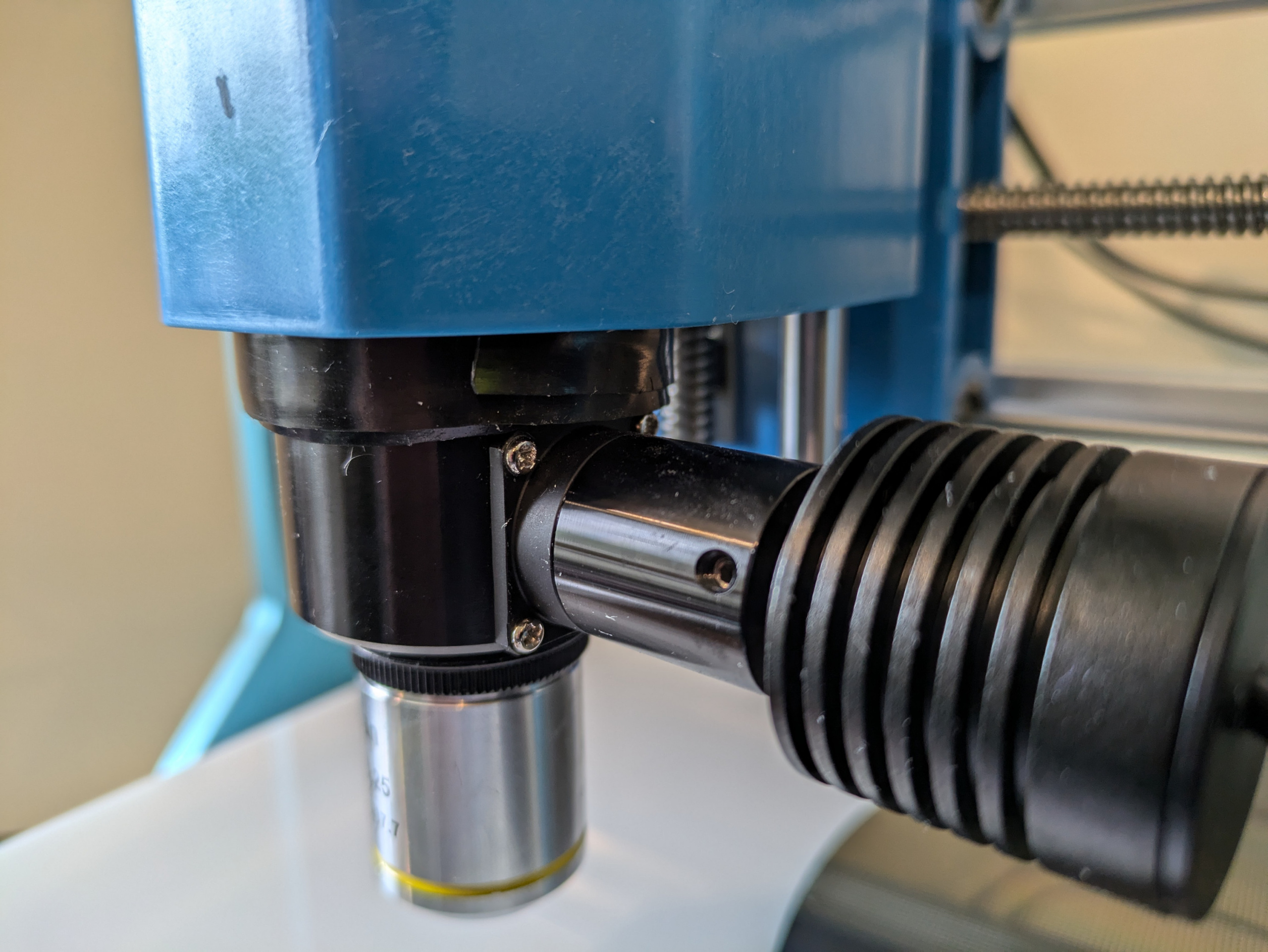
The AmScope imaging sensor was then attached to the C-Mount thread on top of the microscope. It was necessary to rotate the image sensor, to do this I gently unscrewed the screw labelled in the following image and turned the sensor and re-tightened the screws.
An adapter provided by Lapsun was then attached to the RMS thread of the 20x objective and then the objective was screwed into the bottom of the microscope.
The LED light source provided by Lapsun was attached to the light port on the side of the microscope.
Parts and approx. costs
- Genmitsu 3018-PROVer V2 – CNC machine – £216
- Lapsun Microscope – Chose Color: 40X-400X Lens – £240
- Metallurgical Objective – Chose Color: Only 20X Lens – £108
- AmScope MU1803 18MP USB 3.0 – Used – £120
- Black neoprene tape – 0.5mm thick, 50mm height – £15
- Sorbothane discs – used for feet for the CNC machine – £20
- Acrylic block – used to raise sample on CNC stage – 300x180x30mm – £40
Initial imaging
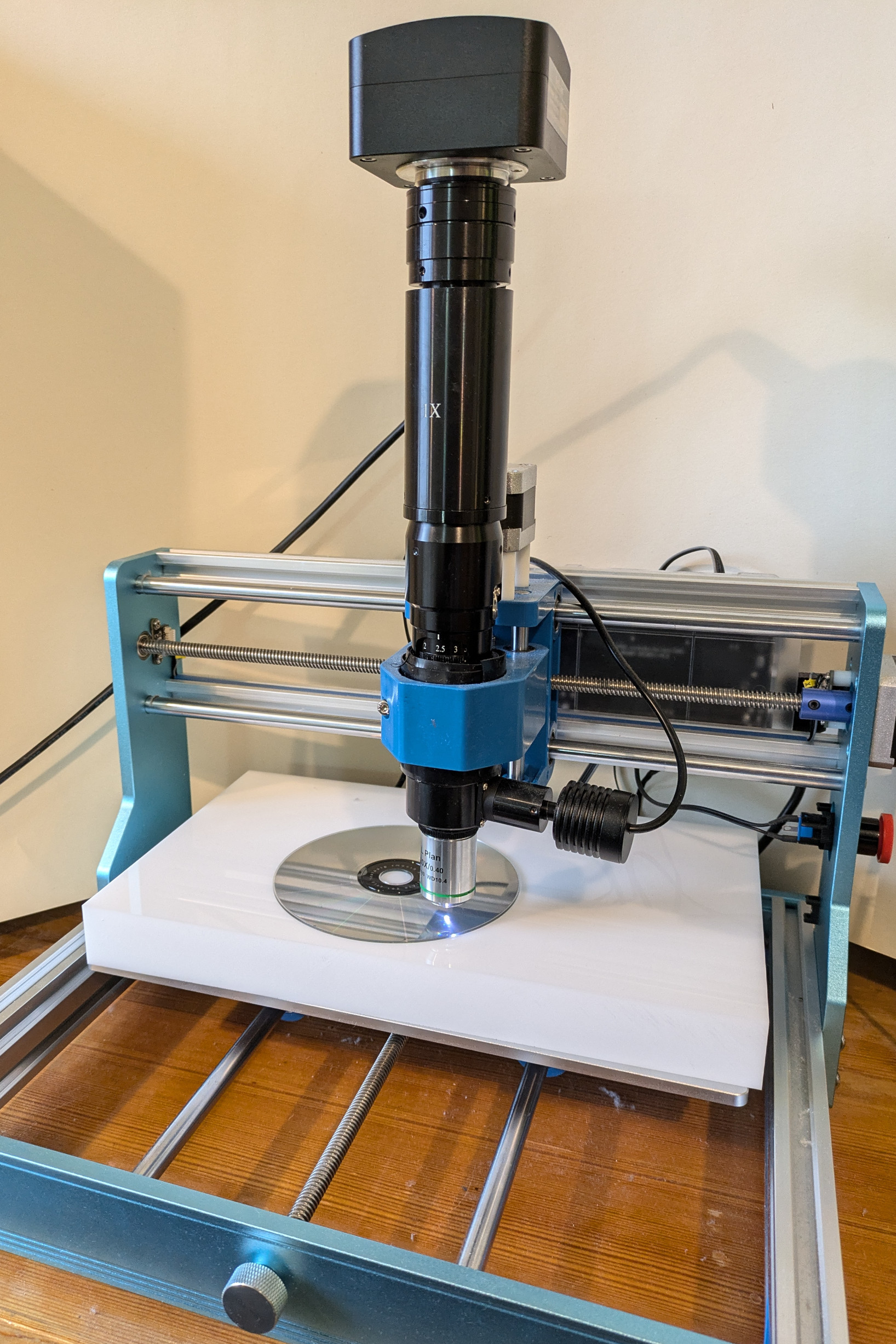
In the following image, you can see the microscope attached to the moveable head of the CNC machine using neoprene tape.
I placed a large cast plastic block onto the CNC stage, so that samples were closer to the microscope (the Z-axis couldn’t reach down far enough for the microscope to image without this).
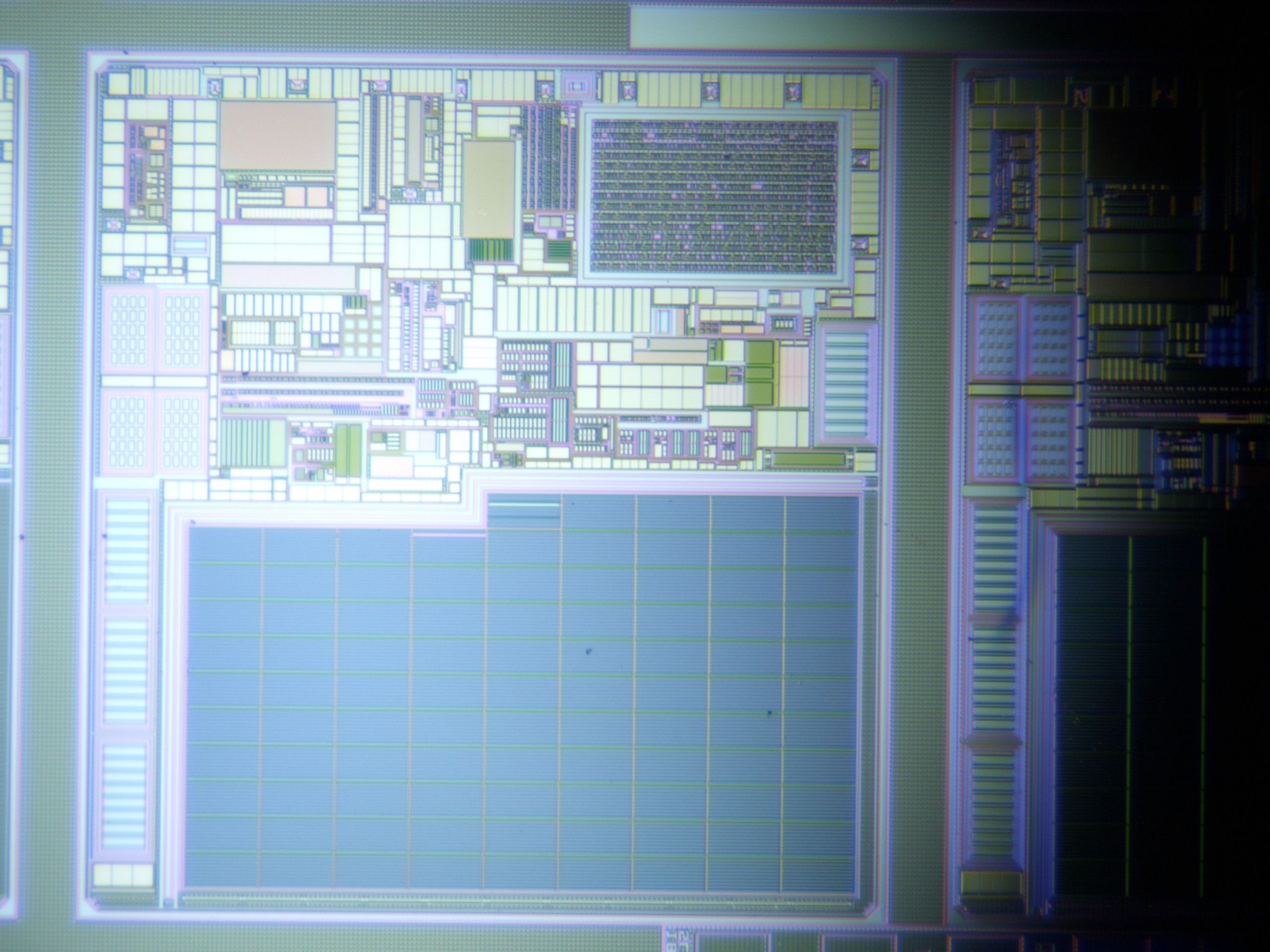
The Z-axis was at -11.798mm to take the first picture from the microscope of a CD-ROM. I then moved the CNC 11cm to the left.
To get from the image shown below, to an in-focus image, I had to adjust the Z-axis upwards to -11.488mm. A difference of 0.31mm.

Magnification
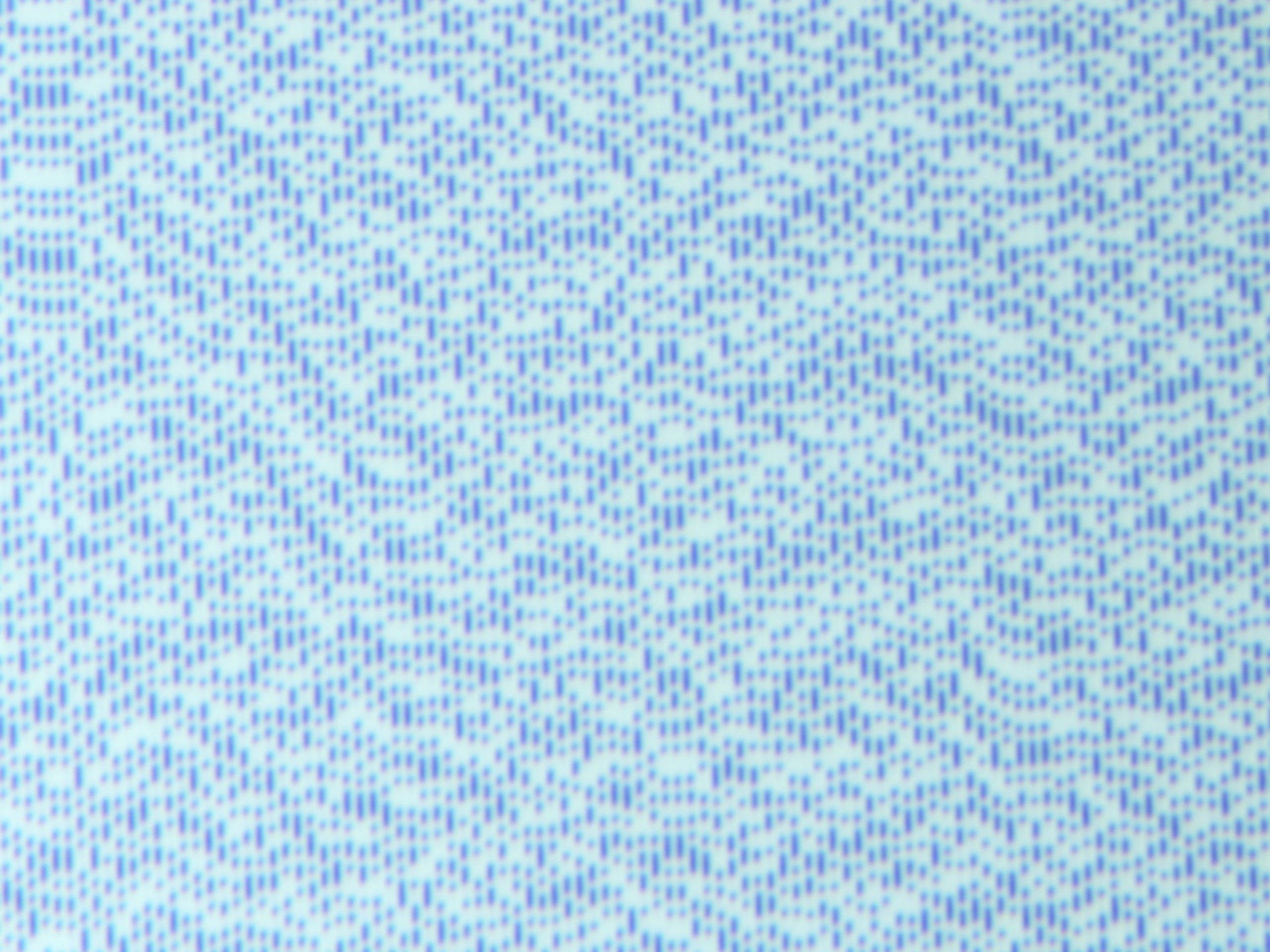
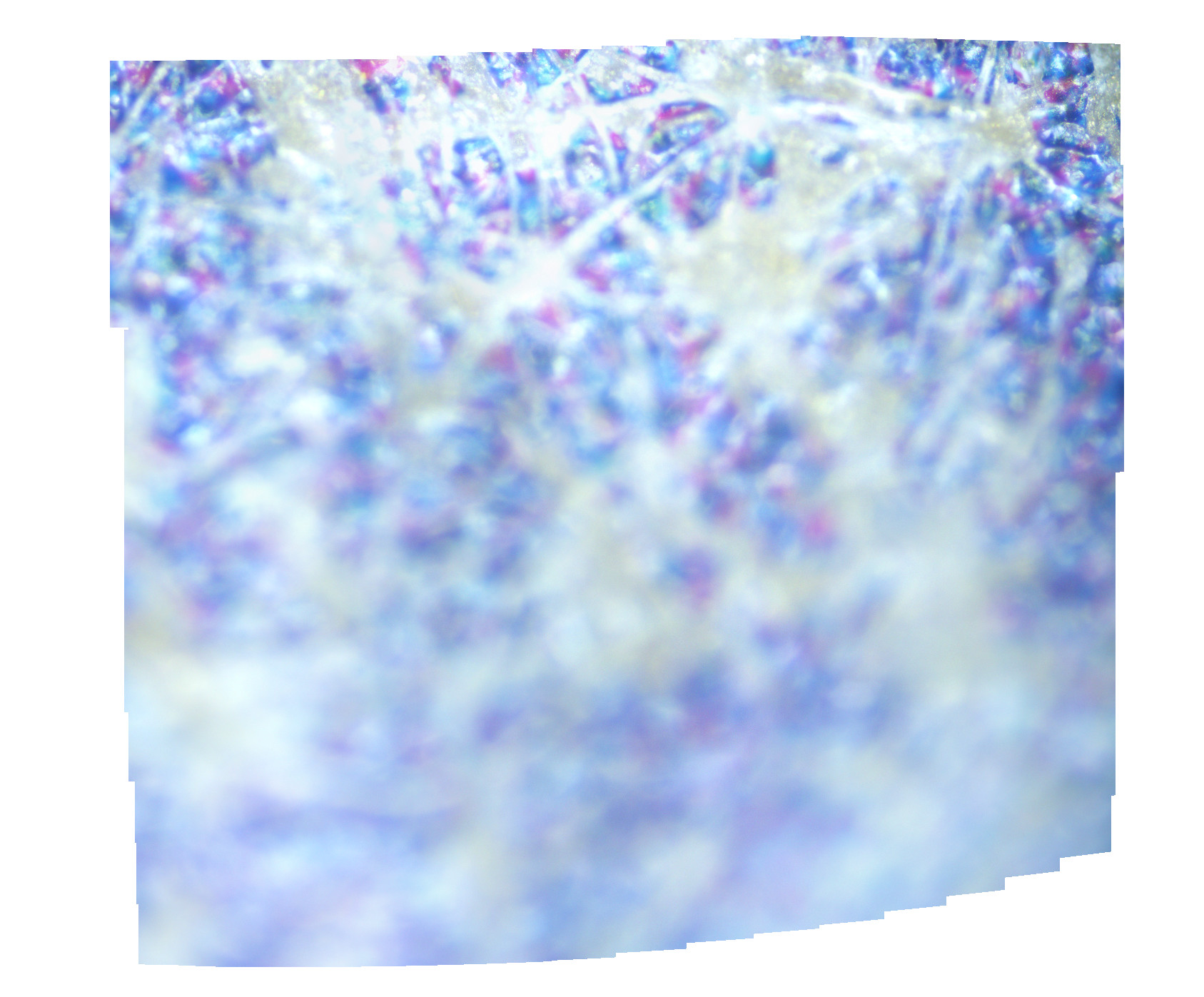
The following image is of white paper with 20x magnification objective and using 4x magnification on the microscope dial.

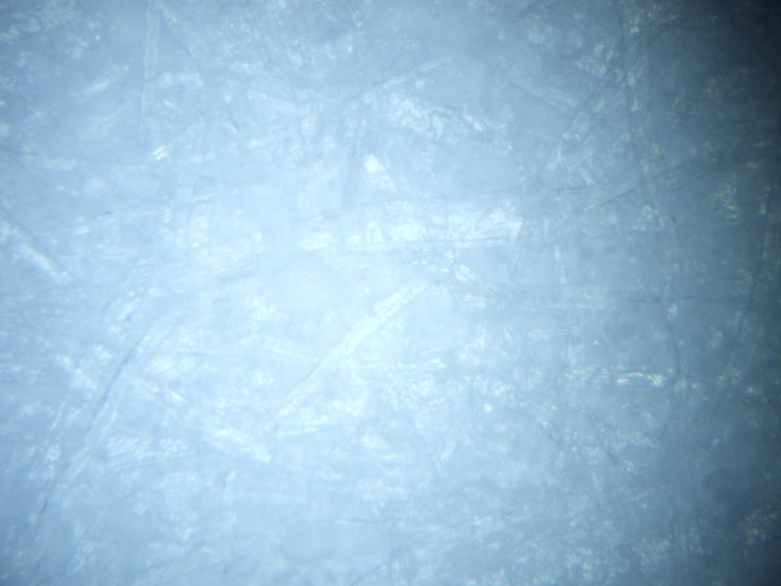
The following image is of white paper with a 20x magnification objective and using 1x magnification on the microscope dial – you can see significant vignetting due to poor illumination (I since found this assumption regarding illumination was incorrect, see below for more information).
After tightening the screws, which you can see in the image below, more properly. The image looks a lot better!

Sharpest regions from a single microscope image
onilink_ (see their website here – http://ic.onidev.fr/en/index.html) suggested to me the great idea of splitting a single microscope image into multiple ’tiles’ and measuring the sharpness of each tile, using the Laplacian of Gaussian – this works since a CD-ROM has a repeating pattern.
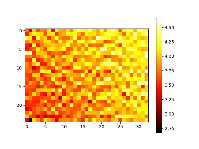
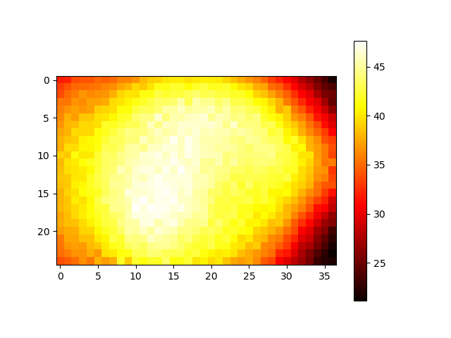
I used the Laplacian function I found from Arducam, but adapted slightly to use ksize=1 , iterated over tiles and generated a heat-map, which you can see below.
The original image has a shape of (3684, 4912) and the number of tiles is (13, 17).
You can see in the heat-map the far right of the image is the sharpest. I’m just hoping this means the CD-ROM is tilted rather than the microscope!
Using a higher quality 10x CD-ROM image from ZeptoBars (see their site https://zeptobars.com/) and the same code, with a tile size of 150. You can see the area of sharpness is in the centre of the image, which makes more sense.
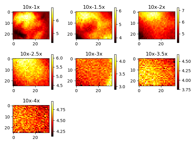
I made a few adjustments – rotating the light source to try to improve light distribution as well as re-tightening the mirror section.
The following shows experiments with CD-ROM images with a 10x objective, with different magnifications on the microscope dial.
The following shows experiments with CD-ROM images with a 20x objective, with different magnifications on the microscope dial.
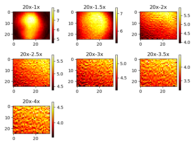
Note that in these previous heatmaps I had manually adjusted the Z height of the microscope to perform focusing.
Software
I created a very simplistic script using Python which you can find at – https://github.com/anfractuosity/cncmicroscopy to automatically capture images from the AmScope camera from x0,y0, to x1,y1 with arbitrary steps.
You can see in the follow image, the pattern that the software generates for the movement of the CNC microscope whilst moving across a sample and capturing images.

I made use of Hugin to stitch the resulting images. following the procedure from – https://hugin.sourceforge.io/tutorials/scans/en.shtml
The first image consists of microscope images of a book cover. You can see how the image becomes more out of focus nearer the bottom. Later in this article I talk about using a simple auto focus algorithm.
Mean Square Error (MSE)
I made use of mean square error to compare pairs of frames for similarity and store these values in a circular buffer. If the standard deviation of this buffer is less than 0.1, I decide the image from the camera has stabilised and so can be used.
I found currently the MSE seems fairly high, due to vibrations being transferred to the table with the microscope on. To lower these I plan to make use of a thick block of granite underneath the microscope as well as removing the CNC machine’s rubber feet and placing sorbothane discs underneath it instead.
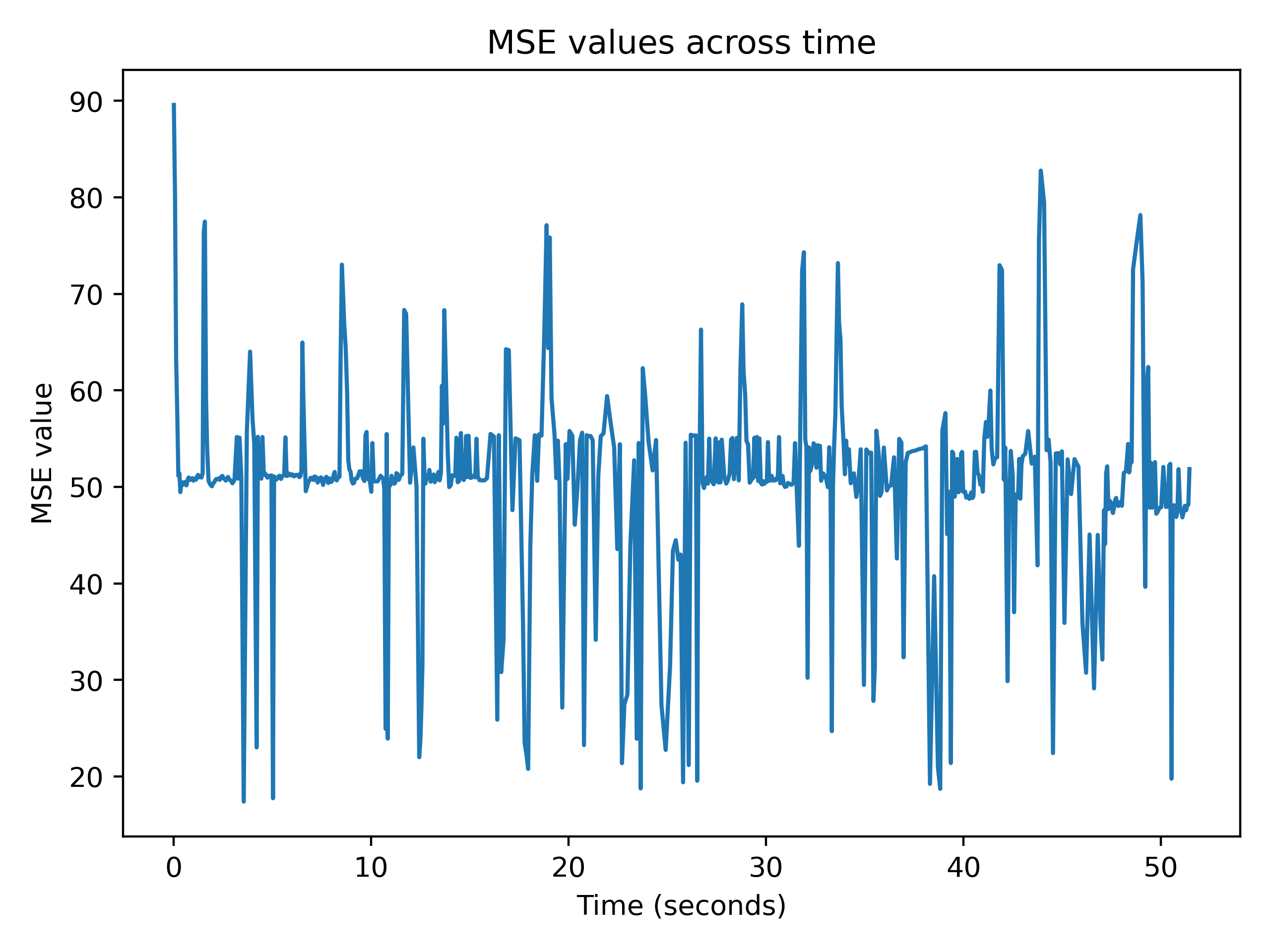
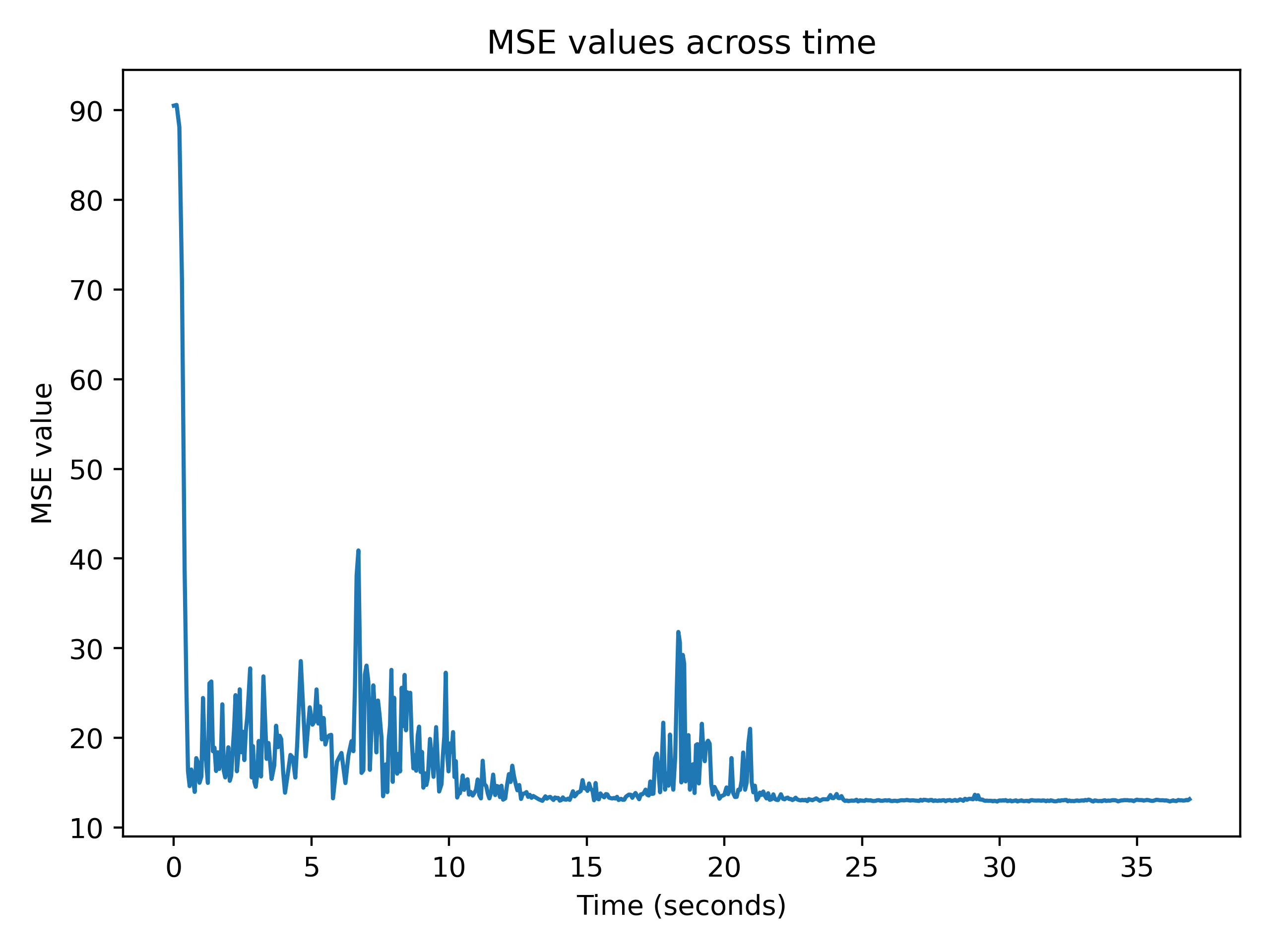
In the following experiments an autofocus procedure is first run. The microscope X axis is then moved 1mm to the right and back 1mm to the left. Then MSE values of pairs of images are created over time and graphed. You can see the MSE value is very high at first at 90, due to the vibrations from the CNC machine itself.
The following graph shows MSE values graphed across time, when external hard disk drives where powered on, on the same desk as the CNC microscope, upstairs.
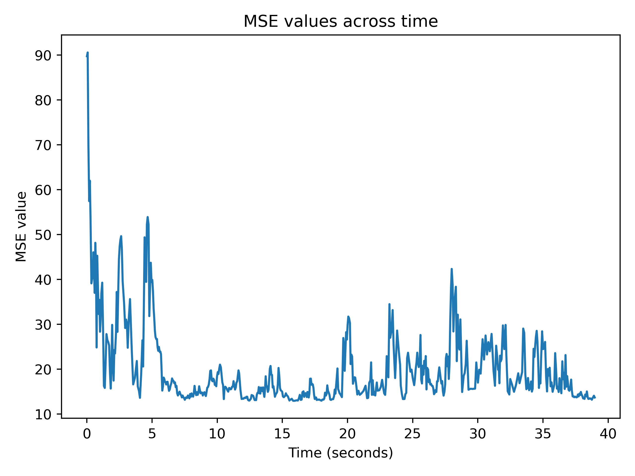
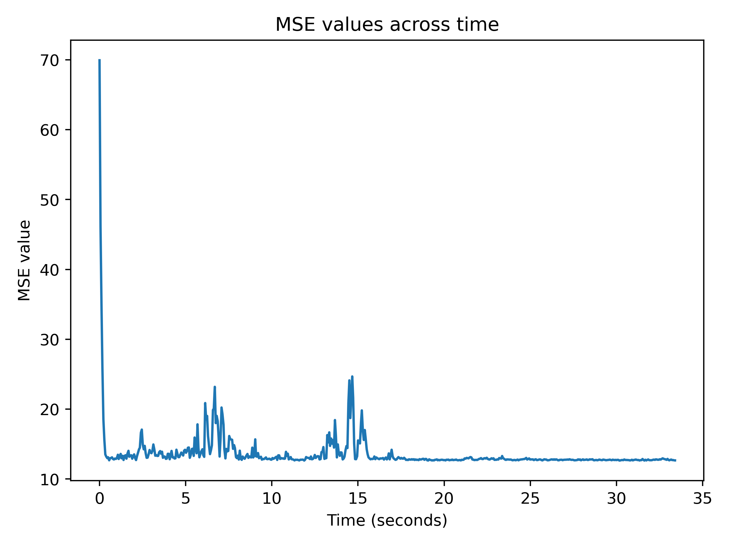
The following graph shows MSE values graphed across time, when external hard disk drives where powered off, on the same desk as the CNC microscope, upstairs.
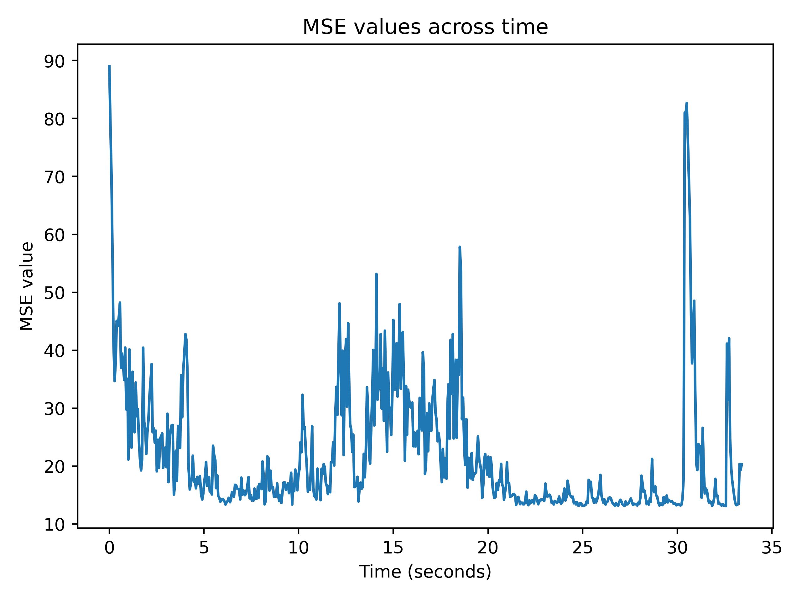
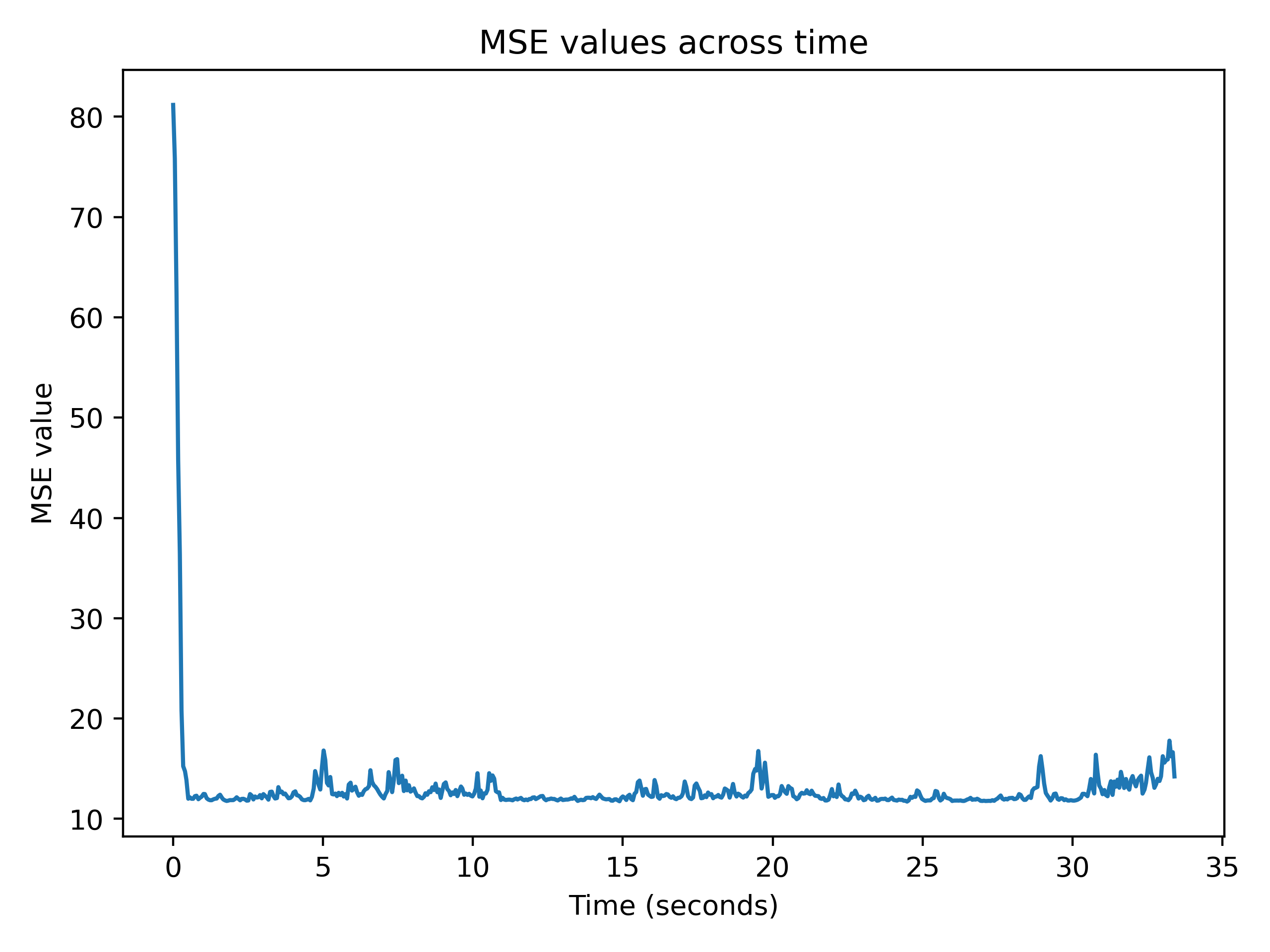
The following shows the same experiment with the CNC machine on the carpet, upstairs.
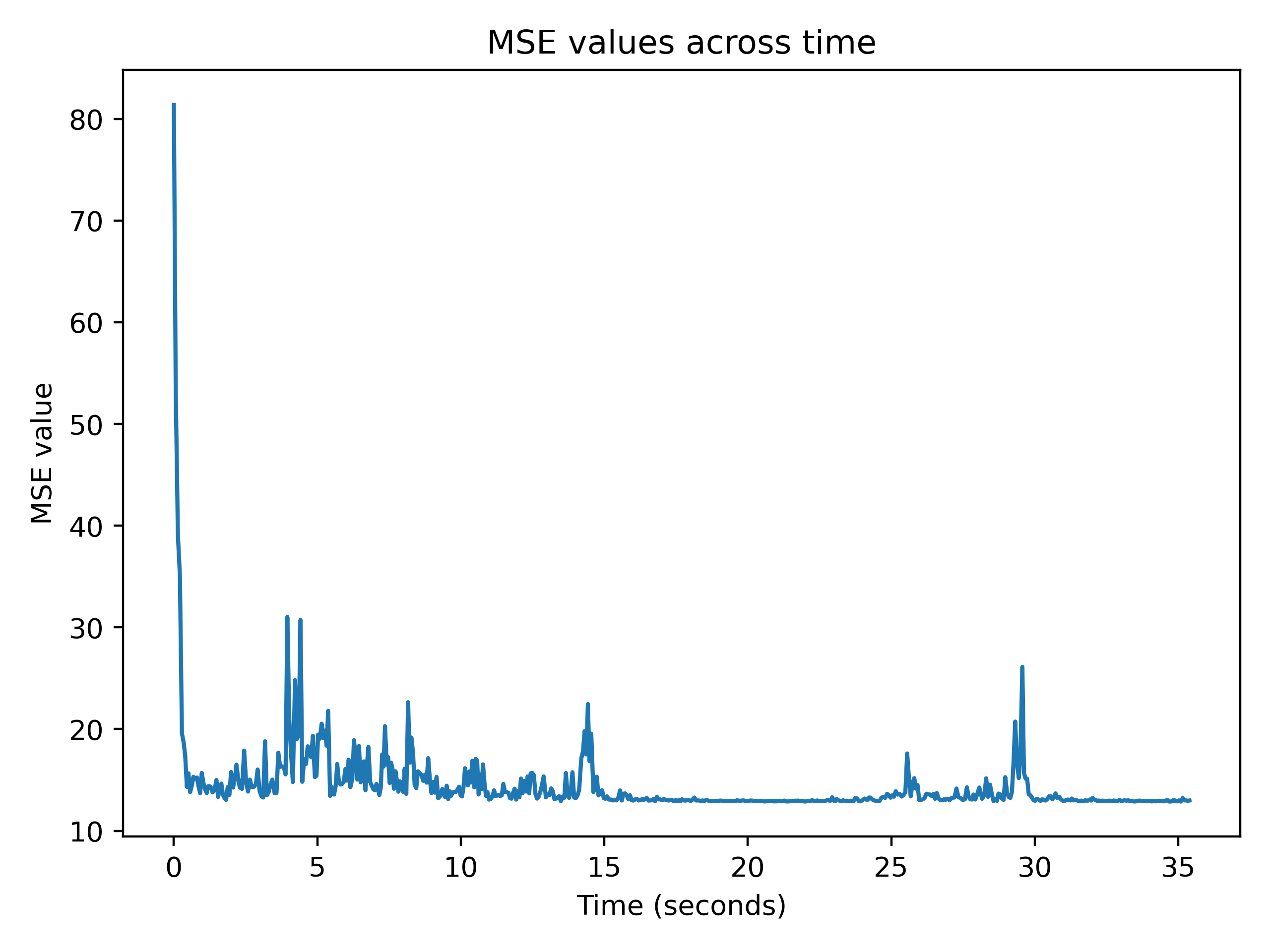
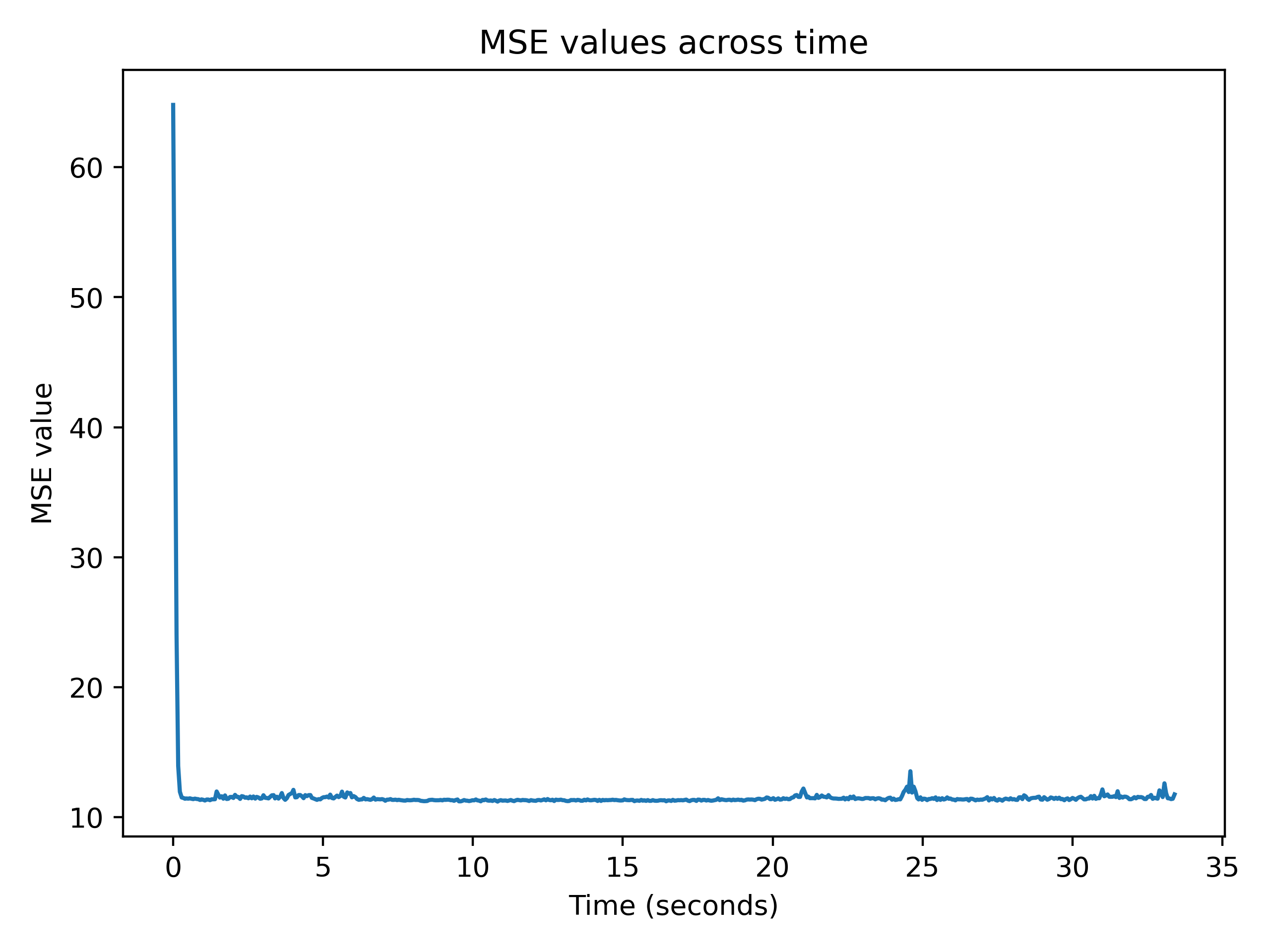
The following shows the same experiment with the CNC machine on the carpet, downstairs.
The following shows the same experiment with the CNC machine on the carpet, downstairs and no rubber feet.
The following shows the same experiment with the CNC machine on the carpet, downstairs and no rubber feet, but adding sorbothane discs.
The following shows the same experiment with the CNC machine downstairs on stone fireplace with no feet.
The following shows the same experiment with the CNC machine downstairs on stone fireplace with no feet but sorbothane discs.
Exposure and framerate
Initially I wasn’t setting the exposure duration manually, but using automatic exposures. I found I was getting only around 3 fps from the camera.
This was significantly improved by dropping the resolution from 4912×3684 to 2456×1842 as well as using manual exposures instead by doing the following:
ctx.hcam.put_AutoExpoEnable(False)
ctx.hcam.put_ExpoTime(ctx.exposure)
ctx.hcam.put_ExpoAGain(100)</pre>
A high framerate is necessary so that MSE can be quickly calculated.
Autofocus
You can see in the following animation, the Z-axis of the CNC machine is adjusted, to adjust focus. It iterates from -10.000 to -12.000mm in steps of 0.01mm. The Laplacian function is used as a method of measuring sharpness.
The video below was generated using the following command:
ffmpeg -framerate 10 -pattern_type glob -i '*.tif' -c:v libx264 out.mp4Stitching
After tiles have been generated it is necessary to stitch them. I initially was using Hugin but then tried Fiji (a distribution of ImageJ2, with lots of plugins).
I needed to flip the images from the camera vertically, so they face the correct direction for stitching. I initially used:
mogrify -flip *.tifI then created a script for Fiji to do this using the stitching plugin. It looks roughly like the below:
run("Grid/Collection stitching", "type=[Filename defined position] order=[Defined by filename         ]
grid_size_x=11 grid_size_y=11 tile_overlap=50 first_file_index_x=0 first_file_index_y=0
directory=/tmp/images file_names=tileb_{x}_{y}.tif output_textfile_name=TileConfiguration.txt
fusion_method=[Linear Blending] regression_threshold=0.30 max/avg_displacement_threshold=2.50
absolute_displacement_threshold=3.50 compute_overlap computation_parameters=[Save memory (but be slower)]
image_output=[Write to disk] output_directory=/tmp/images");
The overlap value itself doesn’t appear to be that important, as compute_overlap appears to calculate this.
I then automated the generation and running of the above ImageJ macro using a simple Python script. It also handles the flipping of images and inversion of the Y axis. I placed this script in the repository for this project, called stitch.py.
I was able to stitch images from an area of 0.5mm x 0.5mm of a CD-ROM, with 0.05mm x/y steps a 20x objective with the microscope tube set to 4x. And obtained a stitched image of 10319×9724, this is shown below, resized and compressed to take up less space. You will notice there appears a slight tilt to the stitched image, this is due I believe to my camera not being perfectly rotated to align with my stage.

I improved the technique from that of the previous approach by using an autofocus algorithm and splitting the area into 0.25mm x 0.25mm squares, within those squares I use steps of around 0.1mm following a ‘snake’ type pattern within the square. Before I capture images within the square, I jump to the mid point of the square (0.25/2=0.125mm, therefore 0.125×0.125mm) and move the Z height from around -11.2m to -11.5mm in 0.001mm steps. At each step I measure the sharpness of the image. I then move above the best Z height, by 0.07mm and iterate from that to beyond the best Z height by 0.07mm. I measure the sharpness again and compare against the best previous sharpness and finish if it’s within 0.5.
I was able to stitch images from an area of 1mm x 1mm of a CD-ROM, with 0.10mm x/y steps a 20x objective with the microscope tube set to 2x.
The stitched image was 10609×10077. I took the stitched image and used the GNU Image Manipulation Program to increase exposure by 2 and reduced both the width and height by 4, so I can present it below.

You will notice there appears a grid like effect. This is due to the lighting not being perfectly uniform throughout the image. To fix this I used the code from stackoverflow. I took an image at -11mm Z height with the same exposure as previous images, but of the blank white plastic surface of my CNC bed and saved that image and was then able to use this algorithm to remove the vignette from my images, before stitching.

You can see the results look much improved.
The following is a crop from the above image, you will notice lines on the right, I believe these may be due to lighting flicker possibly.
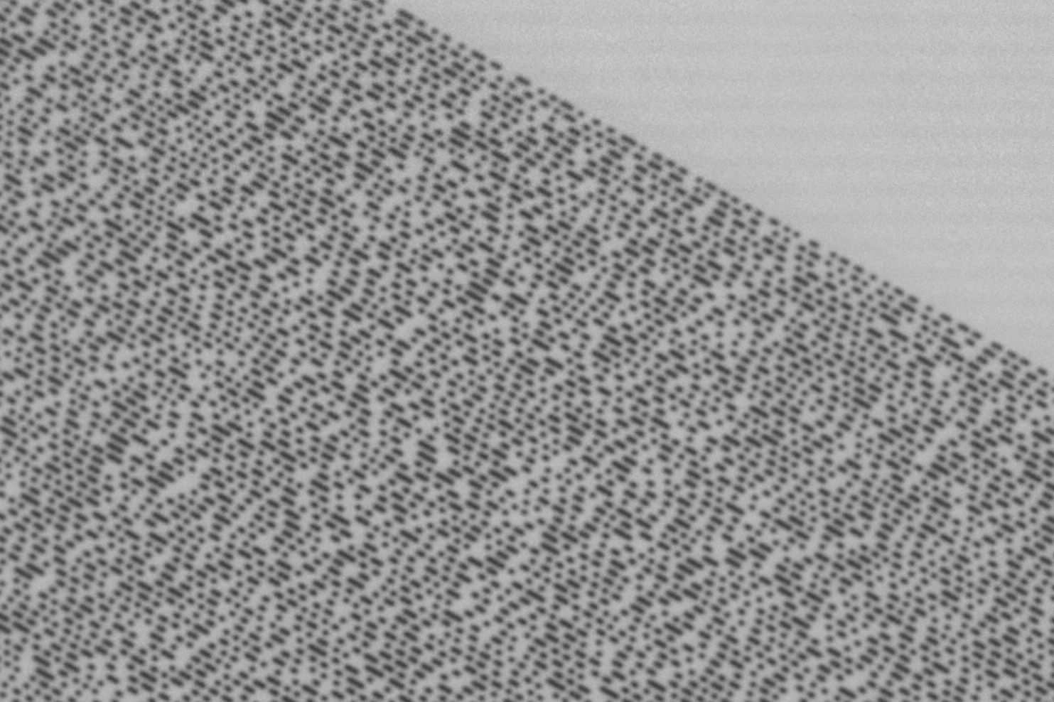
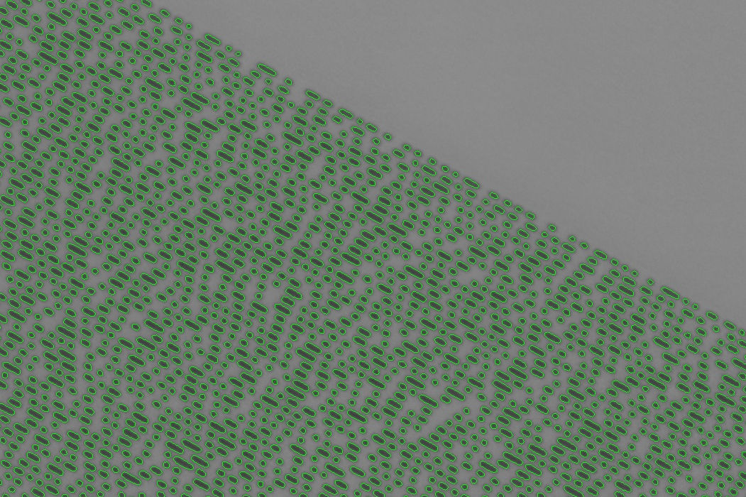
The above image shows contours drawn around the pits.
To Do
- See if kinematic table means I can move 11cm across CD-ROM without having to adjust Z-axis
- Try out focus stacking
DIY solutions
- https://openflexure.org/ – Cool looking DIY 3D printed motorised microscope
- https://github.com/TadPath/PUMA – Another awesome 3D printed microscope
Commercial solutions
The following is a list of some commercial solutions:
- https://www.labsmore.com/ – Lots of cool looking microscopes as well as graphical open source software – https://github.com/Labsmore/pyuscope
- https://meijitechno.com/product/mt8500-m-motorized-metallurgical-microscope/ – Rather pricey (around $44k)
2 Comments
Leave Comment
Error
Rodrigo
It would be really cool if you could do this on a vinyl record, and then see if you could reconstruct the sound. Kind of what they do in the UC Berkeley IRENE project: https://exhibits.lib.berkeley.edu/spotlight/project-irene/feature/the-digitization-process
admin
That’s a cool idea, I’ll have to look if there’s a very small record size I could test it on.